7 Adaptive Resistance in Colorectal Cancer Example

This section contains instructions to reproduce the results of simulating perturbations on FVS control nodes in a network of colorectal cancer (CRC) signaling pathways. The goal of these simulations is to identify targets that can reprogram cells from a MAPK inhibitor therapy resistant phenotype to the MAPK inhibitor therapy sensitive fate. You can read the original report here: link

The original study of reversion of resistance to MAPKi therapy was performed by Park et al. in “Feedback analysis identifies a combination target for overcoming adaptive resistance to targeted cancer therapy (Oncogene volume 39, pages3803–3820 (2020))”. The network and internal-marker nodes were extracted from the publication and its supplementary material. The normalized expression data and mutational profiles used for initial activities in NETISCE was downloaded from the Cancer Cell Line Encyclopedia fromThe Cancer Dependency Map.

The input data, nextflow pipeline, and results of this simulation can be found in the colorectal_cancer_validation folder in the NETISCE github repository

7.1 Input Data

network.sif contains the network structure for CRC signaling

expression.csv contains the initial activities for HT29 untreated cells. The columns for H29_BRAFi (MAPK inhibitor therapy resistant state) and H29_BRAFi+EGRFi (MAPK inhibitor therapy sensitive state) are copies of the HT29 column

internal-marker-1.txt contains the 3 internal marker nodes that were originally used in Park et al., to evaluate simulations.

internal-marker-apoptosis.txt contains the internal marker nodes related to apoptosis used to evaluate simulations.

internal-marker-mapk.txt contains the internal marker nodes related to mapk used to evaluate simulations.

internal-marker-proliferation.txt contains the internal marker nodes related to proliferation used to evaluate simulations.

samples.txt contains they key for NETISCE to associate certain samples to the phenotypes of untreated (HT29), resistant (HT29_BRAFi), and sensitive (HT29_BRAFiEGFRi)

mutations.csv mutational profile of HT29 cells, as well as the overrides for simulating BRAFi and EGRFi.

7.2 Run the simulation

These simulations were run on a high performance cluster that uses a SLURM executor. If your hpc uses a different executor, please update those specifications in the nextflow.config file in the directory. Please see https://www.nextflow.io/docs/latest/config.html for more information regarding your executor.

For ease of reproduction, we have included all files necessary to reproduce the reported results directly in the directory. We highly recommend you run this simulation on an hpc, as you will be generating files of 3Gb+. We have included the bash file we used on our SLURM executor.

Note: within the NETISCE_mutations.nf configuration file, you will want to change the params.internal_control line if you want to use a different set of internal-marker nodes.

#!/usr/bin/env nextflow

params.expressions = "$baseDir/input_data/expression.csv"
params.network = "$baseDir/input_data/network.sif"
params.samples = "$baseDir/input_data/samples.txt"
params.internal_control="$baseDir/input_data/internal-marker-1.txt"
params.mutations="$baseDir/input_data/mutations.csv"
params.alpha = 0.9
params.undesired = 'resistant'
params.desired = 'sensitive'
params.filter ="strict"

As discussed in our paper, we filtered the perturbations using the original 3 internal-marker nodes for apoptosis, proliferation, and MAPK signaling. We further filtered perturbations on the FVS control nodes using 17 addition internal-marker nodes, related to the phenotypes of apoptosis, proliferation, and MAPK signaling. Therefore, to use a set of internal-marker nodes, please point to the correct input-data file. We created folders within the results folder to house the relevant internal-marker node files for each set. You may want to do the same as to not overwrite them (or move them into a separate folder). Additionally, when you run the nextflow command, please be sure to use the -resume flag so that you use the cached computations that do not need to be re-computed

You can run NETISCE directly from this folder using the following command: ./nextflow run NETISC_mutations.nf -resume

7.3 Results

Herein, we will focus on the results that are deposited in the results folder by NETISCE. However, each step of the nextflow pipeline produces its corresponding raw results (for example, the entire attractor state for network simulations initialized with experimental data). If you are interested in looking at those raw results, they can be found within the work folder. We provide workfiles.txt which is a guide to which folders/subfolders contain the relevant results of each step.

7.3.1 General Results

First, let’s take a look at the results that do not depend on the internal-marker node set.

FVS finding

Here we focus on one of the FVSes in the network, which we call, Set 1.

name
AKT1
CCNA1
CTNNB1
E2F1
GRB2
MAPK1
MAPK14
MAPK8
MDM2
PDK1
SMAD7
SRC
TP53
TSC1

Set 1 contains 14 nodes. Notice that TP53 is included in the FVS. This is a mutant gene in HT29 cells. NETISCE_mutations automatically filters out mutated genes, and places the FVS without mutated genes in the fvs-no-mutated-genes.txt file.

and we remove mutated genes!

name
AKT1
CCNA1
CTNNB1
E2F1
GRB2
MAPK1
MAPK14
MAPK8
MDM2
PDK1
SMAD7
SRC
TSC1

Attractor landscape estimation via k-means analysis

Now, let’s look at the results of k-means analysis. First, NETISCE determines the optimal number of k clusters by computing the elbow and silhouette metrics.

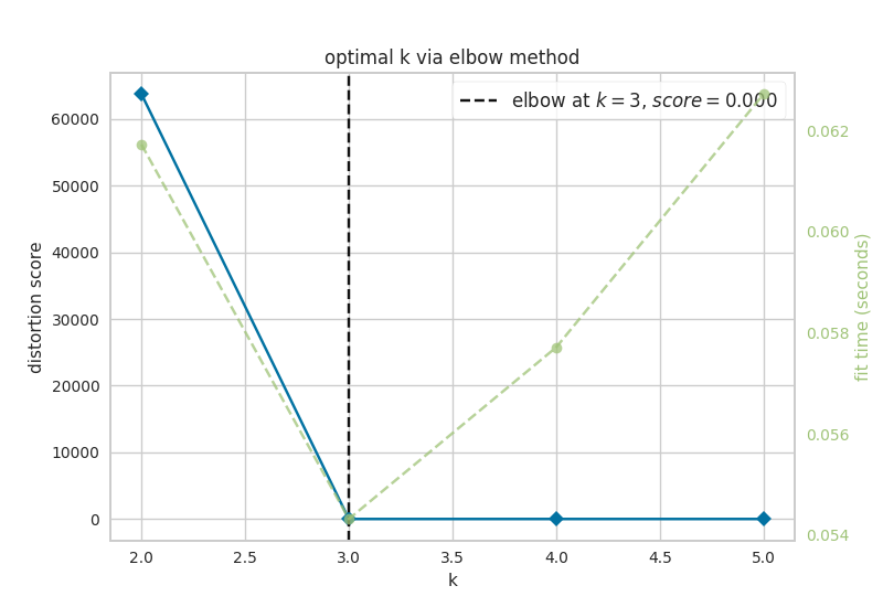
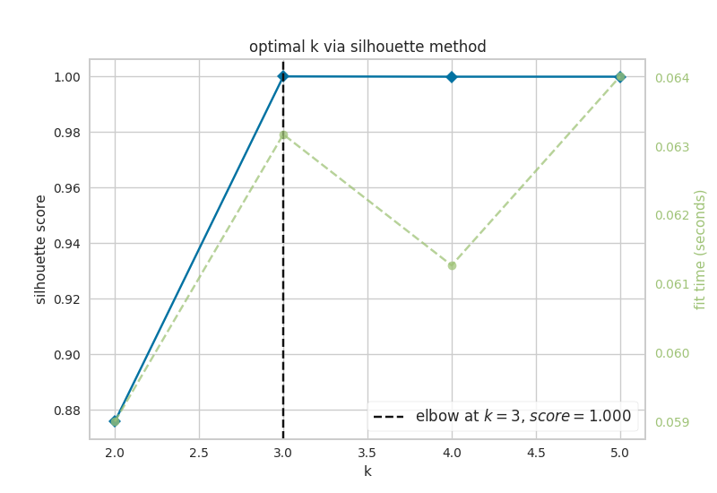
Figure 7.1: optimal k as identified by a) the elbow and b) silhouette metrics

We see that the optimal k assessed by both the elbow metric and silhouette metric was k=3. NETISCE checkes to make sure that the untreated, MAPK inihibitor therapy resistant, and MAPK inhibitor therapy sensitive attractors are all separate.

We can look at those results in the kmeans.txt file.

name	clusters
HT29	0
HT29_BRAFiEGFRi	2
HT29_BRAFi	1

Pertrubations on FVS control nodes that pass criterion 1

With 13 FVS control nodes, NETISCE performed 1,594,323 simulations of combinations of perturbations on the FVS control nodes. The resulting attractors were classified to the clusters produced from the k-means analysis using Naive Bayes, Support Vector Machine, and Random Forest Machine Learning classification algorithms. Then, the perturbations are filtered by which of their corresponding attractors were classified to the MAPK inhibitor therapy sensitive cluster by at least 2 of the 3 methods. These results can be found in crit1_perts.txt. Here we show the first 10 rows.

## [1] "number of perturbations that pass filtering criteria 1: 232114"

x
pert_0
pert_1
pert_2
pert_9
pert_10
pert_11
pert_18
pert_19
pert_20
pert_27

7.3.2 Results using 3 internal-marker nodes

The relevant files have the prefix ‘original’ in the github repository

Our second perturbation filtering criterion identifies perturbations where, in their corresponding attractors, 90% of the steady state values for internal-marker nodes that are within the steady state expression ranges in the attractor representing MAPK inhibitor therapy sensitivity.

First, let’s take a look at the steady state values of the internal-marker nodes CASP3, CCNE1, and MAPK1 in the attractors generated from the untreated HT29 with simulated BRAFi (resistant) and BRAFi+EGFRi (sensitive). The values can be found in the exp_internalmarkers.txt and are plotted in -experimental_internalmarkers.pdf:

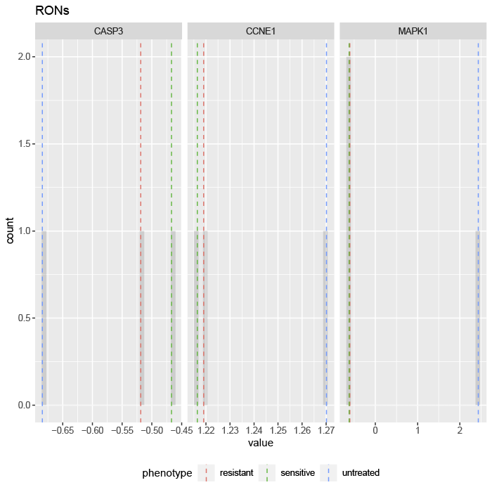
Figure 7.2: histograms of 3 internal-marker node values

We see that the value of the internal-marker for the apoptosis (CASP3) is higher and the steady-state values of the internal-marker nodes for proliferation (CCNE1) and MAPK signaling (MAPK1) are lower in the MAPK inhibitor therapy sensitive associated attractor than the MAPK inhibitor therapy resistance and untreated associated attractors.

Now, we can take a look at the attractors that passed filtering criterion 2. We show the first 10 rows here, but you can view the entire set in successful_controlnode_perturbations.txt

crit2_3<-read.delim('crc/results/3-marker-nodes/successful_controlnode_perturbations.txt',sep=" ",as.is = T)
print(paste0('number of perturbations that pass filtering criteria 2: ',nrow(crit2_3)))

## [1] "number of perturbations that pass filtering criteria 2: 52703"

knitr::kable(crit2_3[1:10,])  %>% column_spec(15, bold = F, border_left = T) %>% scroll_box(width = "100%", box_css = "border: 0px;") 

	AKT1	CCNA1	CTNNB1	E2F1	GRB2	MAPK1	MAPK14	MAPK8	MDM2	PDK1	SMAD7	SRC	TSC1	up	down	total
pert_797158	nochange	nochange	nochange	nochange	nochange	nochange	nochange	nochange	nochange	nochange	nochange	down	nochange	0	1	1
pert_265717	down	nochange	nochange	nochange	nochange	nochange	nochange	nochange	nochange	nochange	nochange	down	nochange	0	2	2
pert_620011	nochange	down	nochange	nochange	nochange	nochange	nochange	nochange	nochange	nochange	nochange	down	nochange	0	2	2
pert_738109	nochange	nochange	down	nochange	nochange	nochange	nochange	nochange	nochange	nochange	nochange	down	nochange	0	2	2
pert_777475	nochange	nochange	nochange	down	nochange	nochange	nochange	nochange	nochange	nochange	nochange	down	nochange	0	2	2
pert_790597	nochange	nochange	nochange	nochange	down	nochange	nochange	nochange	nochange	nochange	nochange	down	nochange	0	2	2
pert_794971	nochange	nochange	nochange	nochange	nochange	down	nochange	nochange	nochange	nochange	nochange	down	nochange	0	2	2
pert_796429	nochange	nochange	nochange	nochange	nochange	nochange	down	nochange	nochange	nochange	nochange	down	nochange	0	2	2
pert_796915	nochange	nochange	nochange	nochange	nochange	nochange	nochange	down	nochange	nochange	nochange	down	nochange	0	2	2
pert_797077	nochange	nochange	nochange	nochange	nochange	nochange	nochange	nochange	down	nochange	nochange	down	nochange	0	2	2

We can look to see if there are any trends in the orientation of the perturbations on FVS control nodes across the perturbations that passed both filtering criteria.

library(data.table)
library(ggplot2)
d3<-crit2_3[,c(1:13)] %>% transpose() %>% as.matrix()
row.names(d3)<-colnames(crit2_3[1:13])
colnames(d3)<-row.names(crit2_3)
d3r<-reshape2::melt(d3) %>% select(-Var2)

#From Paul Tol: https://personal.sron.nl/~pault/
Tol_muted <- c('#88CCEE', '#44AA99', '#117733', '#332288', '#DDCC77', '#999933','#CC6677', '#882255', '#AA4499', '#DDDDDD')

ggplot(d3r, aes(x=value)) +
  facet_wrap(~Var1,scales = "free_x",shrink=FALSE) +
  geom_bar(aes(y = (..count..)/ncol(d3),fill=value))  + scale_y_continuous(labels=scales::percent) + scale_fill_manual(values=Tol_muted)+ ylab("% of specified perturbation to an FVS control node across all \n combinations of perturbations that passed filtering criteria ") + xlab("node perturbation")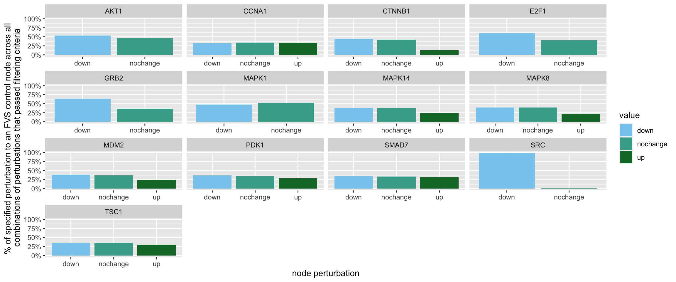

Figure 7.3: the precentage of specific perturbations on FVS control nodes in the perturbations that passed the filtering criteria

Here, we see that in the majority of perturbations, SRC is knocked-out.

The steady-state values of the internal-marker nodes for these perturbations can be found in pert1_internal_markers.txt.

The combination BRAFi+SRCi treatment was identified and experimentally validated by Park et al., to overcome adaptive resistance to MAPK inhibitor therapy in HT29 cells. This perturbation, pert_797158, passed both of our filtering criteria. We can plot the steady-state values of the internal-marker nodes for HT29_BRAFi, H29_BRAFi+EGFRi, and HT29_BRAFi+SRCi using a radar plot.

library(fmsb)
attr_pert<-read.delim("crc/results/3-marker-nodes/pert_internal_markers.txt",sep=" ",row.names = 1) %>% mutate(across(where(is.numeric), ~ round(., digits = 3)))
attr_pert <-attr_pert[c('pert_797158'),]
exp<-read.delim("crc/results/3-marker-nodes/exp_internalmarkers.txt",sep=" ",row.names = 1) %>% mutate(across(where(is.numeric), ~ round(., digits = 3)))
exp<-exp[c(2,3),]

d1<-rbind(exp,attr_pert) 

maxcol<-apply(exp, 2, max)
mincol<-apply(exp, 2, min)
d2<-rbind(maxcol,mincol, exp)
rownames(d2)[1:2]<- c("Max", "Min")
create_beautiful_radarchart(d2,color = c("#00AFBB", "#E7B800","#FC4E07"),caxislabels = seq(min(d2),max(d2),.4),title ="resistant and sensitive attractors");legend(x=0.4, y=1.4, legend =c(row.names(d2)[3:nrow(d2)]) , bty = "n", pch=20 , col=c("#00AFBB", "#E7B800","#FC4E07") , text.col = "black", cex=1, pt.cex=2)

# library(NMF)
# annot<-c("sensitive","resistant","perturbation")
# aheatmap(t(d1),scale="none",Rowv = NA,color = colorRampPalette(c("navy", "white", "firebrick3"))(80), annCol=annot,cellwidth = 30)

rownames(d1)[3]<- c("HT29_BRAFi+SRCi")
maxcol<-apply(d1, 2, max)
mincol<-apply(d1, 2, min)

d2<-rbind(maxcol,mincol, d1)
rownames(d2)[1:2]<- c("Max", "Min")




par(mar = c(4, 0.1, 4, 0.1))
for (i in 5:nrow(d2)) {
  create_beautiful_radarchart(d2[c(1:4, i), ],color = c("#00AFBB", "#E7B800","#FC4E07"),caxislabels = seq(round(min(d2[c(1:4, i),]),1),round(max(d2[c(1:4, i),]),1),.2),title =row.names(d2)[i]);legend(x=0.4, y=1.4, legend =c(row.names(d2)[3:nrow(d2)]) , bty = "n", pch=20 , col=c("#00AFBB", "#E7B800","#FC4E07") , text.col = "black", cex=1, pt.cex=2)
}

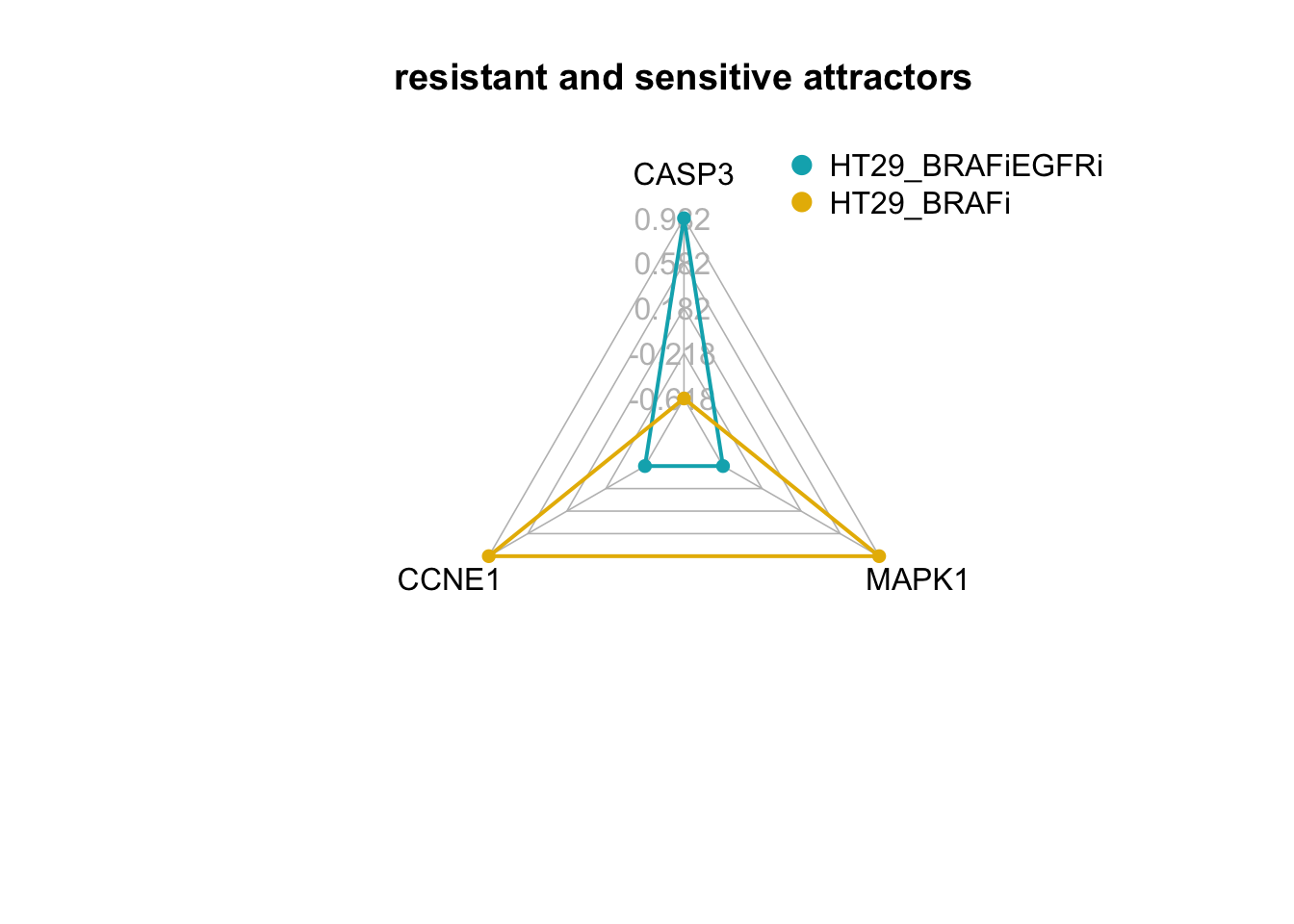
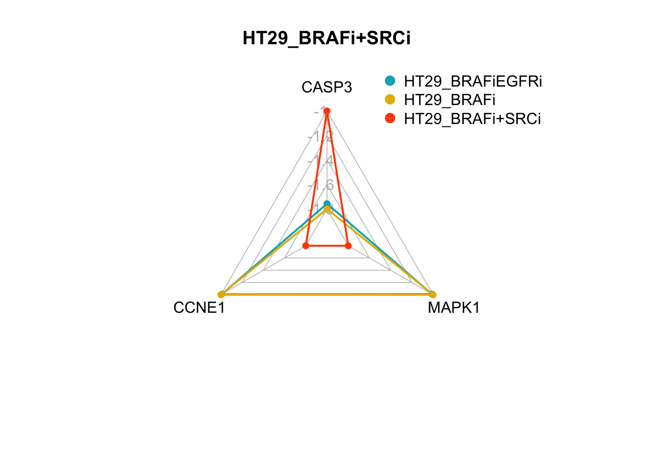
Figure 7.4: radar charts of the steady-state values of 3 internal-marker nodes for HT29_BRAFi+SRCi

We see here that the steady state value of CASP3 in the attractor produced from the HT29_BRAFi+SRCi perturbation is within the range of attractor produced from the HT29_BRAFi+EGFRi perturbation.

7.3.3 Results using apoptosis, proliferation, and MAPK signaling internal-marker nodes

We filtered the 52,703 perturbations using an additional 17 internal-marker nodes for the phenotypes of apoptosis, proliferation, and mapk signaling.

The individual results for all three sets can be found in their respective folders on github: apoptosis-marker-nodes mapk-marker-nodes proliferation-marker-nodes

We are interested in perturbations on FVS control nodes that pass the filtering criterion for each of the three phenotypes (i.e., the 90% threshold for steady-state values is met separately for each of the sets of apoptosis, MAPK signaling, and proliferation nodes). We can plot the node perturbation trends for these perturbations.

allthree<-crit2_3[c(Reduce(intersect, list(row.names(crit2_3),row.names(crit2_apop),row.names(crit2_prolif),row.names(crit2_mapk)))),]
print(paste0('number of perturbations that pass filtering criteria 2: ',nrow(allthree)))

## [1] "number of perturbations that pass filtering criteria 2: 1266"

d4<-allthree[,c(1:13)] %>% transpose() %>% as.matrix()
row.names(d4)<-colnames(allthree[1:13])
colnames(d4)<-row.names(allthree)
d4r<-reshape2::melt(d4) %>% select(-Var2)



ggplot(d4r, aes(x=value)) +
  facet_wrap(~Var1,scales = "free_x",shrink=FALSE) +
  geom_bar(aes(y = (..count..)/ncol(d4),fill=value))  + scale_y_continuous(labels=scales::percent)+
  theme(panel.spacing.x = unit(4, "mm")) + scale_fill_manual(values=Tol_muted) + ylab("% of specified perturbation to an FVS control node across all \n combinations of perturbations that passed filtering criteria ") + xlab("node perturbation")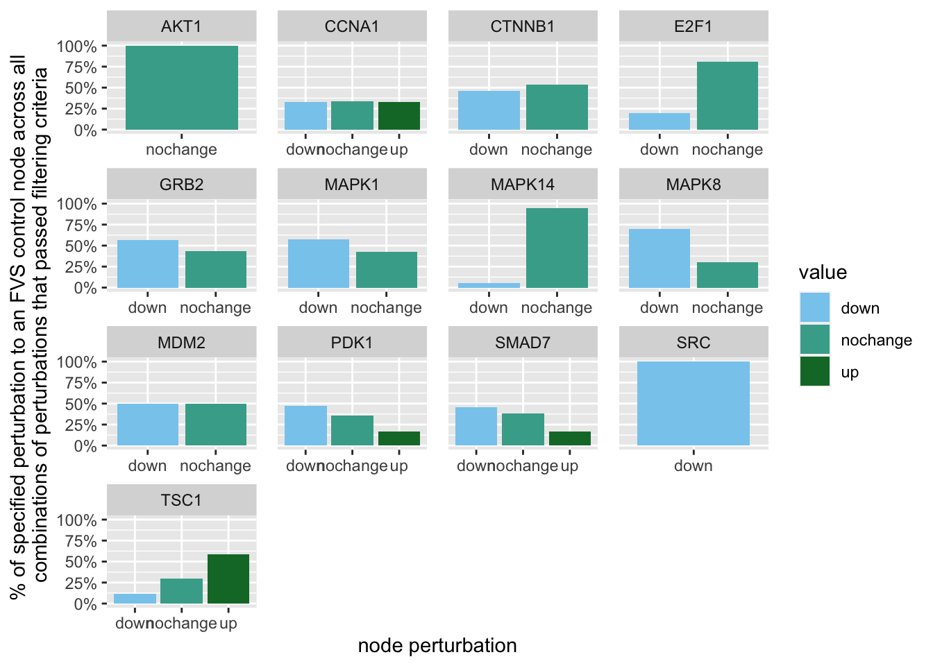

Figure 7.5: the precentage of specific perturbations on FVS control nodes in the perturbations that passed the filtering criteria

For perturbations that pass the 2nd filtering criterion using internal-marker nodes for apoptosis, MAPK sigaling and proliferation, we see that in 100% of the perturbations SRC is downregulated. In the majority of of perturbations, TSC1 is upregulated, and GRB2 is downregulated.

The two smallest sets of perturbations that passed the filtering criteria were BRAFi+SRCi+TSC1overexpression (pert_797159) and BRAFi+SRCi+GRB2i (pert_790597). We can make radar charts for each phenotype’s internal marker nodes to show that the steady-state values for the internal marker-nodes produced from these perturbations are within the gene expression range of the MAPK inhibitor therapy sensitivty assocaited attractor (HT29_BRAFi+EGFRi).

attr_pert<-read.delim("crc/results/apoptosis-marker-nodes/pert_internal_markers.txt",sep=" ",row.names = 1)
attr_pert <-attr_pert[c('pert_797159','pert_790597'),]
exp<-read.delim("crc/results/apoptosis-marker-nodes/exp_internalmarkers.txt",sep=" ",row.names = 1)
exp<-exp[c(2,3),]

d1<-rbind(exp,attr_pert)

rownames(d1)[3:4]<- c("HT29_BRAFi+SRCi+TSCovr","HT29_BRAFi+SRCi+GRB2i")
maxcol<-apply(d1, 2, max)
mincol<-apply(d1, 2, min)

d2<-rbind(maxcol,mincol, d1)
rownames(d2)[1:2]<- c("Max", "Min")

par(mar = c(4, 0.1, 4, 0.1))
for (i in 5:nrow(d2)) {
  create_beautiful_radarchart(d2[c(1:4, i), ],color = c("#00AFBB", "#E7B800","#FC4E07"),caxislabels = seq(round(min(d2[c(1:4, i),]),1),round(max(d2[c(1:4, i),]),1),.2),title =row.names(d2)[i]);legend(x=0.4, y=1.4, legend =c(row.names(d2)[c(3,4,i)]) , bty = "n", pch=20 , col=c("#00AFBB", "#E7B800","#FC4E07") , text.col = "black", cex=1, pt.cex=2)
}

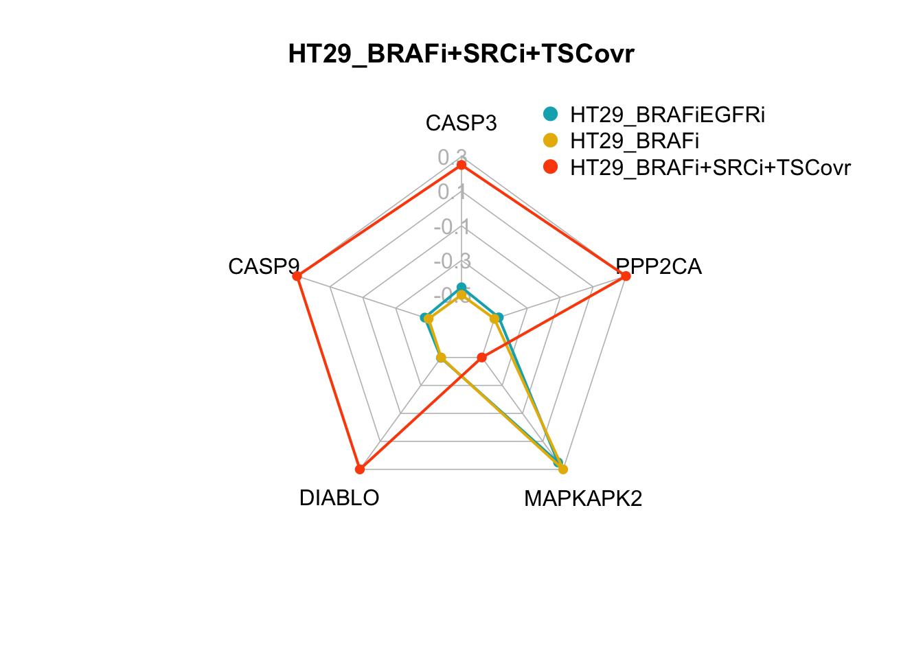
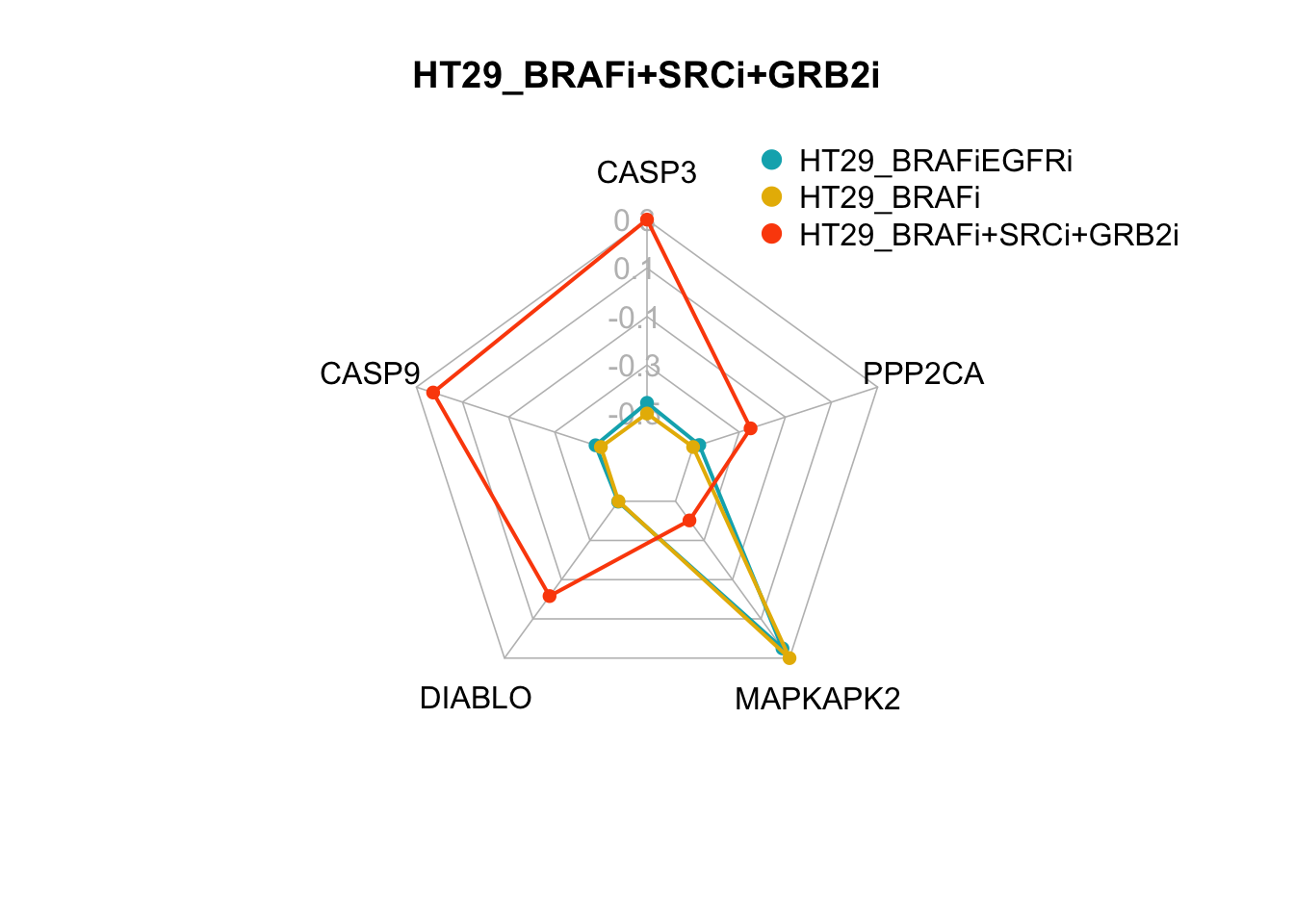
Figure 7.6: radar charts of the steady-state values of apoptosis internal-marker nodes for HT29_BRAFi+SRCi_TSCovr and HT29_BRAFi+SRCi_GRB2i

attr_pert<-read.delim("crc/results/mapk-marker-nodes/pert_internal_markers.txt",sep=" ",row.names = 1)
attr_pert <-attr_pert[c('pert_797159','pert_790597'),]
exp<-read.delim("crc/results/mapk-marker-nodes/exp_internalmarkers.txt",sep=" ",row.names = 1)
exp<-exp[c(2,3),]

d1<-rbind(exp,attr_pert)

rownames(d1)[3:4]<- c("HT29_BRAFi+SRCi+TSCovr","HT29_BRAFi+SRCi+GRB2i")
maxcol<-apply(d1, 2, max)
mincol<-apply(d1, 2, min)

d2<-rbind(maxcol,mincol, d1)
rownames(d2)[1:2]<- c("Max", "Min")

par(mar = c(4, 0.1, 4, 0.1))
for (i in 5:nrow(d2)) {
  create_beautiful_radarchart(d2[c(1:4, i), ],color = c("#00AFBB", "#E7B800","#FC4E07"),caxislabels = seq(round(min(d2[c(1:4, i),]),1),round(max(d2[c(1:4, i),]),1),.2),title =row.names(d2)[i]);#legend(x=0.4, y=1.4, legend =c(row.names(d2)[c(3,4,i)]) , bty = "n", pch=20 , col=c("#00AFBB", "#E7B800","#FC4E07") , text.col = "black", cex=1, pt.cex=2)
}

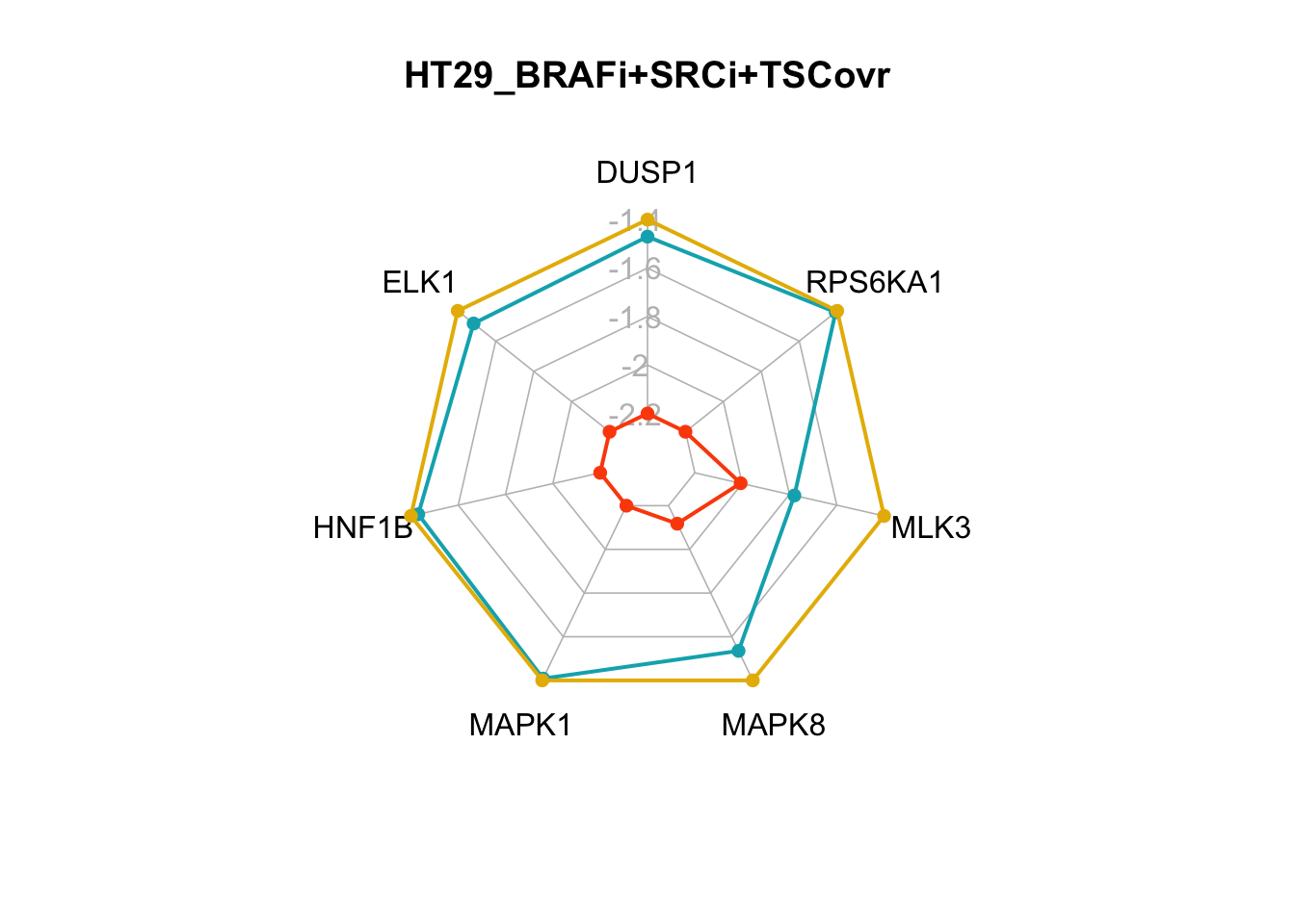
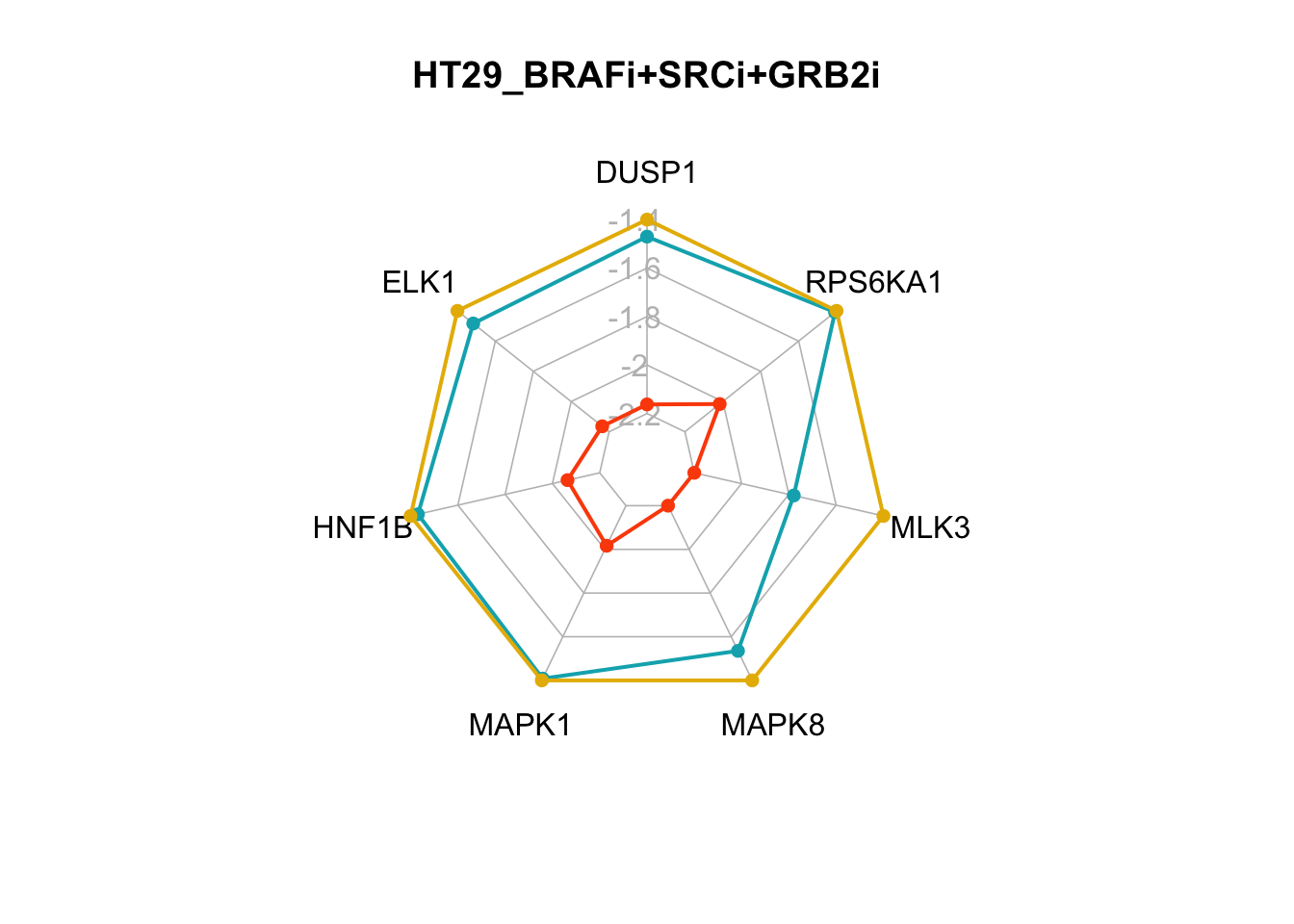
Figure 7.7: radar charts of the steady-state values of MAPK signaling internal-marker nodes for HT29_BRAFi+SRCi_TSCovr and HT29_BRAFi+SRCi_GRB2i