4 Toy Network Examples

Here, we will walk through a brief tutorial of a NETISCE run. The files necessary to complete the tutorial are within the input data folder of both NETISCE_local and NETISCE_hpc. The results from these Toy examples can be found in the toy_example_results folder of the main github repository.

4.1 Overview

We will use a simple toy network of 6 nodes and 9 edges.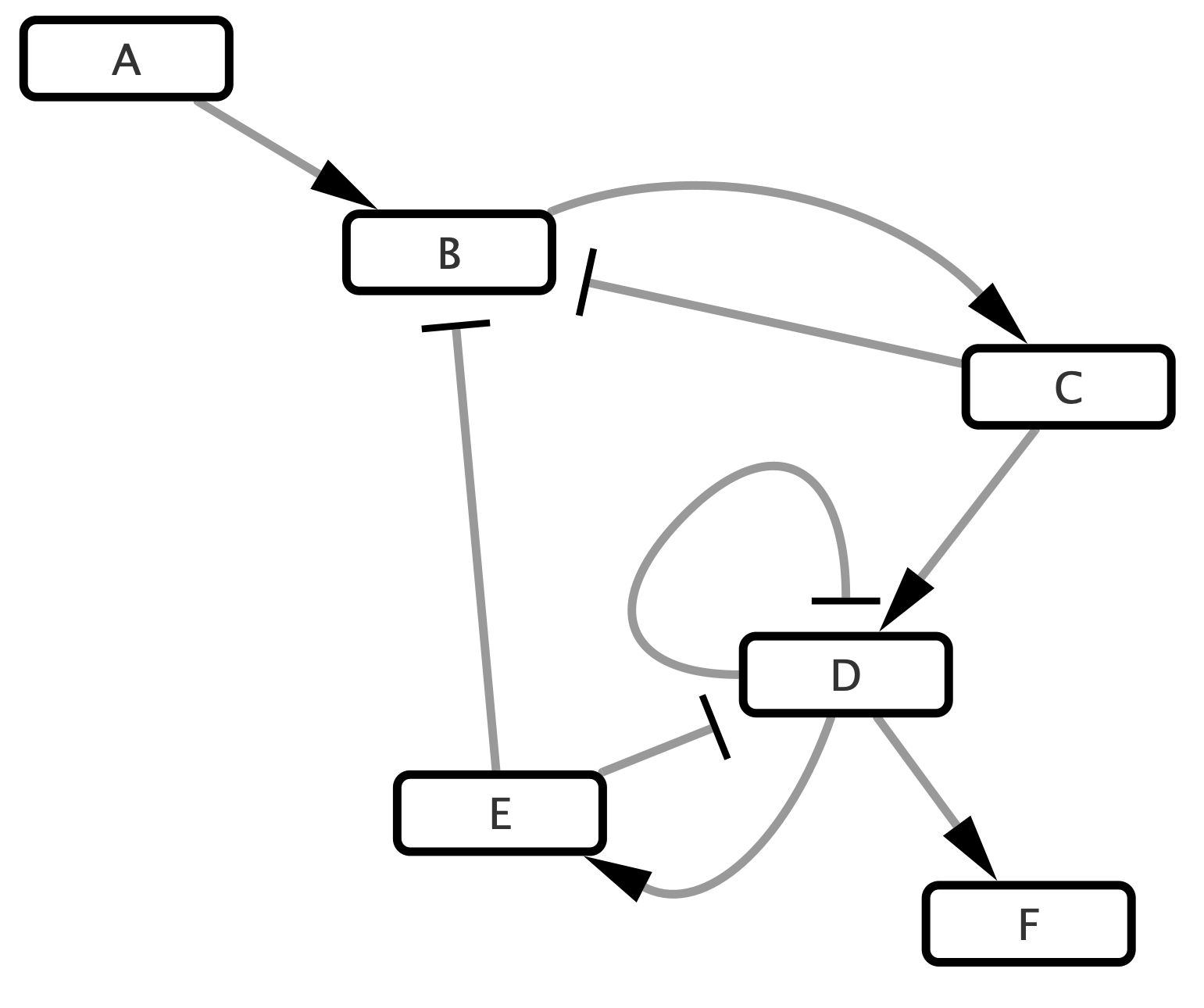

Figure 4.1: Simple Toy Network

4.2 Data

You can find the relevant data files in the input_data folder.

In this example, we have 2 samples, A and B, with three replicates each (A_1,A_2,A_3, etc). The normalized expression data is housed in expressions.csv, and contains normalized expression values for the network nodes. Note that the value of F has been initialized to zero. A feature of NETISCE is that it does not require non-zero values for all network nodes, which is useful if the data is unavailable for a node. Such values can either be entered in the expressions.csv file as 0s, or the node can be excluded entirely from this file, depending on user preference (in this case, the values will automatically be initialized to 0).

X	A_1	A_2	A_3	B_1	B_2	B_3
A	2	1	2	6	7	6
B	6	7	6	2	1	1
C	5	5	5	1	1	1
D	-1	-1	-2	6	7	6
E	2	1	2	6	7	6
F	0	0	0	0	0	0

The samples.txt file specifies that A is associated to a treatment sensitive phenotype, while B is associated to a resistance phenotype.

sample_name	phenotype
A_1	sensitive
A_2	sensitive
A_3	sensitive
B_1	resistant
B_2	resistant
B_3	resistant

Note that you can use any term to describe the phenotypes. Just be sure to be consistent with the param.desried and param.undesired variables within the Nextflow .nf file.

Lastly, we need to include a list of internal marker nodes. This list is in internal_marker.txt. For our small network, the internal-marker node is C.

C

4.3 NETISCE run configuration

With all your input data files loaded, next we configure the nextflow run in either NETISCE_local or NETSICE_hpc (Note: while we do recommend you run NETISCE on a hpc, this example is small enough to run locally).

Open up NETISCE.nf. Here, you need to specify the parameters for the Nextflow run on lines 3-19. Please refer to section 2.5 for parameter definitions.

For this example, your parameters should look like:

params.expressions = "$baseDir/input_data/expressions.csv"
params.network = "$baseDir/input_data/network.sif"
params.samples = "$baseDir/input_data/samples.txt"
params.internal_control="$baseDir/input_data/internal_marker.txt"
// params.mutations="$baseDir/input_data/mutations.csv"
params.alpha = 0.9
params.undesired = 'resistant'
params.desired = 'sensitive'
params.filter ="strict"


params.kmeans_min_val = 2
params.kmeans_max_val = 10


params.num_nodes = 6 // that have expression data
params.num_states = 100000

params.randseed=0

Some Notes: make sure to include $baseDir before pointing to the folder containing your input data. Also, be sure that params.num_nodes is the number of nodes where there exists data within expressions.csv. Finally, by adjusting the params.randseed you can identify alternate FVSes within the nextwork.

4.4 Run NETISCE

In your terminal/command prompt, navigate to the appropriate NETISCE folder (_hpc or local). To start your run, enter ./nextflow run NETISCE.nf -resume. While NETISCE is running, your terminal should look like this, where you can see the progress on each step of the pipeline:

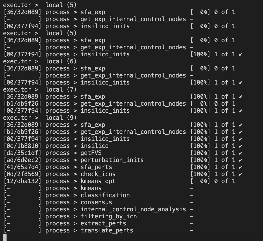
Figure 4.2: Terminal when running NETISCE

The first column contains the location (folder and subfolder) that is running that step of NETISCE within the work folder.

Once the run has successfully completed, the process will end and the following will be displayed:

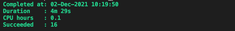
Figure 4.3: Terminal when running NETISCE

4.5 NETSICE Results

Let’s take a look at the results of our NETISCE run, where the goal was to shift the system from the undesired state B, and towards the desired state A. These results can be found in the toy_example_1 subfolder of the toy_example_results folder of the main github repository.

exp_internalmarkers.txt

Our internal marker node was node C. In this file we see the steady state values of node see in the A sample replicates A_1, A_2 and A_3 and B sample replicates B_1, B_2, and B_3 (as computed by SFA).

name	C
A_1	0.792
A_2	0.844
A_3	0.800
B_1	0.232
B_2	0.171
B_3	0.166

experimental_internalmarkers.pdf

The above numbers may be a little challenging to read! So, we have included a plot of the values in theexperimental_internalmarkers.pdf:

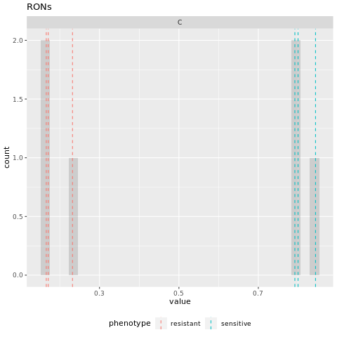
Figure 4.4: experimental marker node steady state values

On this histogram, we see bars for each of the samples and their replicates. The A (sensitive) samples are marked by a blue vertical line at their steady state value, while the B (resistant) samples are marked by a red vertical line at their steady state value. The grey bars can be aggregated to show the number of attractors with values for C that are binned together (for example, in the above table we see that the steady state value of C in replicate B_2=0.171 and replicate B_3=0.166. These values are binned together on the histogram to show that two replicates had similar values.)

Here, we see that the values of node C are well separated between the two phenotypes (all of the A values are greater than all of the B values). We will assume that this also aligns with the biological knowledge of the system.

After estimating attractors for the experimental and randomly generated initial states, the resultant attractors were clustered using k-means clustering. The elbow and silhouette metrics are used to determine the optimal number k.

elbow.png

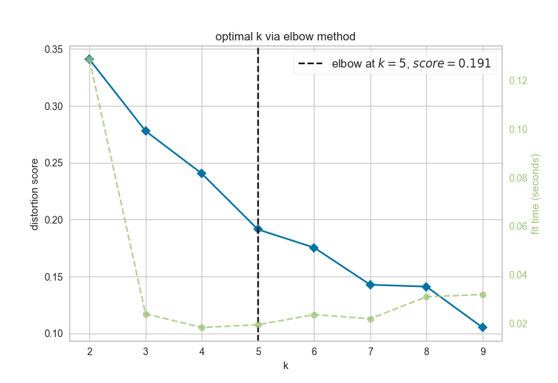
Figure 4.5: elbow metric for optimal k

The elbow metric found the optimal number of k clusters to be k=5.

silhouette.png

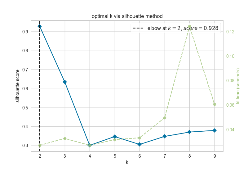
Figure 4.6: silhouette metric for optimal k

The silhouette metric found the optimal number of k clusters to be k=2.

Since the optimal ks identified by the silhouette metric and the elbow metric do not match, NETISCE chooses the smaller k, as long as the phenotypes remain separate (NETISCE checks to make sure this is true).

kmeans.txt

The kmeans.txt file contains the clustering results for each attractor generated from the experimental data and the randomly generated initial states. The first column contains the sample name, and the second column contains the ID of which cluster it is assigned to. Since k=2 in this case, one cluster is named “0” and the other cluster is named “1”

name	clusters
A_1	0
A_2	0
A_3	0
B_1	1
B_2	1
B_3	1

And we see in the kmeans.txt file, that the A samples are clustered in cluster 0, while the B samples are grouped in cluster 1.

4.5.0.1 FVS_Finding output of FVSes.txt

The FVS_Finding Nextflow script was used to identify all unique FVSes in the toy network.

V1	V2	V3
FVS_0	B	E
FVS_2	C	D
FVS_5	B	D
FVS_11	C	E

The first column contains the FVS identifier, where the number is the randomseed value where that FVS was identified. There were four FVSes identified in this network, each comprised of two nodes (column2 and column 3)

fvs.txt

We selected FVS_0 to be analyzed in this example. Therefore, params.randomseed was set to 0

name
B
E

The FVS finding algorithm identified nodes B and E to be a minimal FVS control nodes in the toy network. Since the FVS control node set contained 2 nodes, 9 combinations of perturbations were performed on the control node sets.

crit1perts.txt

This file contains a list of IDs for the perturbations to FVS control nodes that passed criterion 1.

V1
pert_0
pert_3
pert_6
pert_7
pert_8

5 out of the 9 perturbations passed the machine learning filtering criterion.

pert_replicate_1_internal_markers.txt

NETISCE calculated perturbations on FVS control nodes when the system was initialized from the three undesired B replicates (B_1,B_2,B_3). The steady state values of the internal marker node C was extracted from each of these replicate perturbations that passed filtering criterion 1 (i.e., the steady state value of C in pert_0, pert_3, pert_6, pert_7, pert_8). Here we will show the steady state values of C under FVS perturbations when the system was initialized with the normalized expression values of B_1 (contained in the file pert_replicate_1_internal_markers.txt; the values of C for the system under perturbations when initialized from B_2 are found in pert_replicate_2_internal_markers.txt, the values of C for the system under perturbations when initialized from B_3 are found in pert_replicate_3_internal_markers.txt )

name	C
pert_0	-2.600000
pert_3	2.657829
pert_6	6.400000
pert_7	6.400000
pert_8	6.400000

successful_controlnode_perturbations.txt

This file contains a table of the perturbations on FVS control nodes that passed both the 1st and 2nd filtering criteria. it also contains the number of upregulation,downregulations, and total number of nodes perturbed for each perturbation set.

	B	E	up	down	total
pert_3	nochange	down	0	1	1
pert_7	up	nochange	1	0	1
pert_6	up	down	1	1	2
pert_8	up	up	2	0	2

Here, we see that four perturbations that passed both filtering criteria.

Let’s take a quick look at the steady state values for these perturbations, and the attractors generated from the experimental data:

	name	C
1	A_1	0.792000
2	A_2	0.844000
3	A_3	0.800000
4	B_1	0.232000
5	B_2	0.171000
6	B_3	0.166000
21	pert_3	2.657829
31	pert_6	6.400000
41	pert_7	6.400000
51	pert_8	6.400000

Indeed, we see that the steady-state expression values of node C in the attractors generated by peturbations to the FVS control nodes are all are greater than the steady-state expression values of node C in the attractors generated from the sensitive A sample. A successful reprogramming from resistant (B) to sensitive (A) cells has occurred!

4.6 Toy Example with mutations

Let’s say that in our system, gene D exhibits a gain of function mutation in the sensitive phenotype (A samples). If we want to include this in our simulations, we will use the NETISCE_mutations.nf pipeline.

First, we must add to our input_data folder a .csv file containing the mutational profile. Let’s call this file mutations.csv:

X	D
A_1	1
A_2	1
A_3	1
B_1	NA
B_2	NA
B_3	NA

The gain of function mutation is encoded with 1 (loss-of-function mutations can be encoded with “0”).

Next, we make sure that the parameters in NETISCE_mutations.nf on lines 3-19 are set correctly for the conditions

For this example, your parameters should look like:

params.expressions = "$baseDir/input_data/expressions.csv"
params.network = "$baseDir/input_data/network.sif"
params.samples = "$baseDir/input_data/samples.txt"
params.internal_control="$baseDir/input_data/internal_marker.txt"
params.mutations="$baseDir/input_data/mutations.csv"
params.alpha = 0.9
params.undesired = 'resistant'
params.desired = 'sensitive'
params.filter ="strict"


params.kmeans_min_val = 2
params.kmeans_max_val = 10


params.num_nodes = 4 // that have expression data
params.num_states = 1000

Note, the additional parameter params.mutations that points to the mutations.csv.

As above, to run Netisce, enter ./nextflow run NETISCE.nf -resume.

Results

By including mutational information, the results of NETISCE have changed.These results can be found in the toy_example_2 subfolder of the toy_example_results folder of the main github repository. Now, our successful_controlnode_perturbations.txt file contains pert_7 in addition to perturbations pert_3, pert_6, and pert_8

	B	E	up	down	total
pert_3	nochange	down	0	1	1
pert_7	up	nochange	1	0	1
pert_6	up	down	1	1	2
pert_8	up	up	2	0	2

Let’s take a look at the steady-state expression values of node C in the attractors generated from the successful perturbations and the experimental initial states B_1 when mutational information is included.

name	C
pert_3	2.319659
pert_6	6.400000
pert_7	6.400000
pert_8	6.400000

Though the values are different in this system with mutations, we still see that the steady-state expression values of node C in the attractors generated by peturbations to the FVS control nodes are all are greater than the steady-state expression values of node C in the attractors generated from the sensitive A sample. A successful reprogramming from resistant (B) to sensitive (A) cells has occurred!